diffusioncma¶

A python/C++ package for calculating diffusion and free energy profiles in anisotropic media.

The algorithms employed to calculate optimal profiles are loosely based on the Bayesian Analysis by Gerhard Hummer and An Ghysels, as implemented in the mcdiff python package: mcdiff. Changes with respect to mcdiff are listed later.

Free software: GNU General Public License v3
MacOS and Linux
Python 3

When using diffusioncma, please cite 1.

Getting started¶

Get Anaconda.

Create and activate a new conda environment, e.g.:

conda create -n dcma_py36 python=3.6
source activate dcma_py36

(Note that you have to activate the environment each time you open a new terminal.) Install the code from anaconda:

conda install diffusioncma -c conda-forge

Try to run the executable:

dcma --help

To compile the code (e.g. when you want to make changes), check out the section about compiling.

If you want to work on the C++ code, check out the instructions to set up diffusioncma as a QtCreator project.

If you experience any errors, feel free to contact me or report an issue on gitlab.

How it Works¶

Input¶

The program takes one or more transition matrices as input. These matrices have to be generated before starting the optimization – this step is currently not supported by the diffusioncma package.

To obtain a transition matrix, the simulation domain is divided into equally-spaced bins \(b_i\) and a lag time \(\tau\) is defined. Compare simulation snapshots \(r(t)\) and \(r(t+\tau)\) and count the numbers of permeants that have transitioned from \(b_j\) to \(b_i\). Sum these transition counts over the whole trajectory and you obtain the transition matrix \(T=(t_ij)_ij\).

(We have a custom CHARMM command (tmat) in our lab that does all this stuff; contact us if you are interesting in using our Fortran code for the tmat command.)

Take a look into the examples directory to see how transition matrices are formatted (the formatting is inherited by mcdiff).

Modeling and Optimization¶

The optimization of the profiles is done with the command:

dcma opt

See the help message for details:

dcma opt --help

The theory underlying the optimization assumes that the permeant dynamics on the lag time scale \(\tau\) are well described by diffusion on a potential energy surface, i.e. a Smoluchowski diffusion equation.

We are now seeking to identify the free energy and diffusion profiles that explain the observed transition counts in the most plausible manner. This is done via a maximum-likelihood estimation. A log-likelihood function is optimized using an efficient derivative-free optimization method, the Covariance Matrix Adaptation-Evolution Strategy (CMA-ES) 5.

The diffusion and free energy profiles are represented by certain basis functions, in order to keep the dimension of the optimization problem and the amount of required sampling tenable. The code supports cosine functions (recommended), cubic splines, and piecewise constant (compartmental) functions. The free energy profile can also be kept constant throughout the optimization.

Output¶

The output contains the permeability according to the inhomogeneous solubility-diffusion model, the optimal profiles, and the resistivity of each bin.

Postprocessing Tools¶

Extrapolation to Infinite Lag Times¶

One difficulty of the Bayesian approach is concerned with chosing the right lag time. Generally, lag times should be chosen so that transitions between different bins occur frequently. However, too long a lagtime will likely blur the local shape of the free energy profile. Conversely, too short a lag time will more likely capture inertial movements and render the dynamics non-diffusive.

A remedy to this dilemma is offered by chosing multiple lag times and obtaining the optimal profiles for each lag time. These optimal profiles can then be extrapolated to \(\tau=\infty\), cf. Ghysels et al. (2017) 4. Diffusioncma supports this extrapolation by the command:

dcma x2inf

Plotting¶

Profiles can be plotted by the command:

dcma plot

Averaging Profiles and Retrieving Errors¶

Statistics (averages and quantiles) of profiles, e.g. for different simulations/replicas of the same system, can be obtained via:

dcma stats

Example: Oxygen in a POPC bilayer¶

To see the interplay of these commands, let us consider oxygen permeation through a POPC bilayer as an example 4. Go into the examples directory:

cd examples/oxygen

The transition matrices for four different replicas A, B, C, D (50 ns per replica) are located in the tmat directory.

Let’s optimize the profiles for replica A using 10 and 6 cosine basis functions for the free energy and diffusion profile, respectively (these are the default settings):

dcma opt tmat/tmat.100bins.A.20.txt -o profiles.A.20.txt

After less than a minute the optimization should be finished. The output file contains the permeability in the first line, the range of bins over which the permeability was calculated in the second, and the profiles afterwards.

We can now also run the optimization for the other lag times:

for tau in 30 40 50; do
    dcma opt tmat/tmat.100bins.A.${tau}.txt -o profiles.A.${tau}.txt;
done;

Let us now extrapolate the profiles to infinite lag times using the command:

dcma x2inf profiles.A.?0.txt -l 20,30,40,50 -o profiles.A.inf20-50.txt

and plot the result:

dcma plot profiles.A.*.txt -o profiles.A

Note that the plotting functionalities might suffer if you do not use latex on matplotlib. (My ~/.matplotlib/matplotlibrc on MacOS looks like this; on Linux the location of the matplotlibrc is ~/.config/matplotlib/matplotlibrc)

Finally, the optimization, extrapolation, and plotting should be run for the other replicas:

for rep in B C D; do
    for tau in 20 30 40 50; do
        dcma opt tmat/tmat.100bins.${rep}.${tau}.txt -o profiles.${rep}.${tau}.txt;
    done;
    dcma x2inf profiles.${rep}.?0.txt -l 20,30,40,50 -o profiles.${rep}.inf20-50.txt;
    dcma plot profiles.${rep}.*.txt -o profiles.${rep};
done;

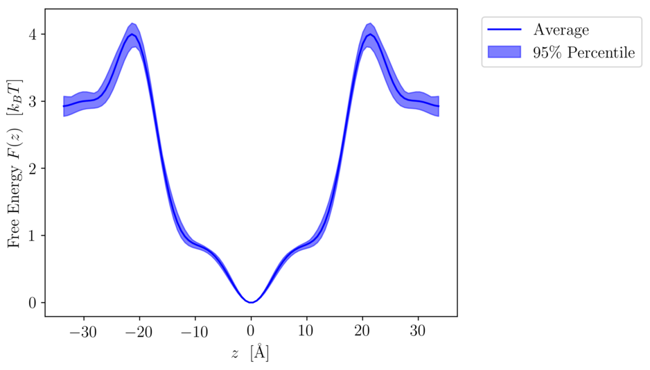
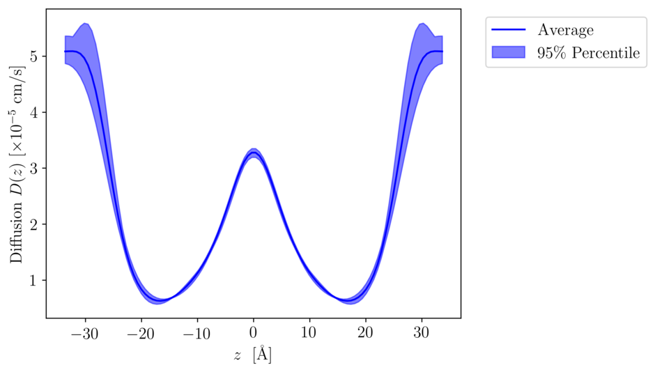
Let us take a look at the statistics of all profiles with “infinite” lag time:

dcma stats profiles.?.inf20-50.txt -o profiles.stats

When calculating the statistics (averages and 95% quantiles), they get plotted automatically. The plots should look pretty much like this:

Changes With Respect to MCDiff¶

Algorithms: The Monte Carlo sampling is replaced by a derivative-free optimization method called CMA-ES.
Efficiency: C++ is used for the computationally expensive parts of the calculations.
Convenience: The vectors containing diffusion profiles in MCDiff store the values at bin edges. Instead, diffusioncma stores the values at the bin centers (consistent with the free energy). When assembling the rate matrix, this is accounted for (the diffusion values that go into the rate matrix are averages over the adjacent bins (i) and (i+1)).

To Be Done / Limitations¶

All models assume periodic boundary conditions.
So far, the code works only for the Smoluchowski equation in one coordinate.
The spline model is flawed due to a bug in the Eigen spline module, which does not really allow to set the gradients to zero at the boundaries of the domain in older versions (see here). Without these boundaries, the splines look kind of weird.

Credits¶

started in May 2018 by Andreas Krämer, Laboratory of Computational Biology (LCB), NHLBI/NIH, Bethesda, MD 1 2
based on previous work by Gerhard Hummer 3 and An Ghysels 4

Diffusioncma uses the following packages:

libcmaes (https://github.com/beniz/libcmaes) by Emmanuel Benazera – CMA-ES Optimizer
pybind11 (http://pybind11.readthedocs.io) by Jakob Wenzel – Python Bindings
lbfgspp (http://yixuan.cos.name/LBFGSpp/) by Yixuan Qui – Quasi-Newton Optimizer (not supported from Python)
Eigen – Linear Algebra in C++
CMake – Compile Workflow
Pytest – Testing the python interface
Click – Python command line interface
numpy/scipy – Linear Algebra in Python
matplotlib – Plotting in Python
Boost (optional) – C++-only command line interface, C++ tests (very coarse-grained testing)

References¶

1(1,2): Andreas Krämer, A. Ghysels, E. Wang, R.M. Venable, J.B. Klauda, B.R. Brooks, R.W. Pastor (2020): Membrane Permeability of Small Molecules from Unbiased Molecular Dynamics Simulations [submitted to J. Chem. Phys.].
2: Richard M. Venable, A. Krämer, R.W. Pastor: Molecular Dynamics Simulations of Membrane Permeability, Chemical Reviews 119 9 (2019) 5954-5997.
3: Gerhard Hummer, Position-dependent diffusion coefficients and free energies from Bayesian analysis of equilibrium and replica molecular dynamics simulations, New J. Phys. 7 (2005) 34. http://stacks.iop.org/1367-2630/7/i=1/a=034.
4(1,2,3): An Ghysels, R.M. Venable, R.W. Pastor, G. Hummer, Position-Dependent Diffusion Tensors in Anisotropic Media from Simulation: Oxygen Transport in and through Membranes, J. Chem. Theory Comput. 13 (2017) 2962–2976. doi:10.1021/acs.jctc.7b00039.
5: Nikolaus Hansen, A. Ostermeier, Completely Derandomized Self‐Adaptation in Evolution Strategies, Evol. Comput. 9 (2001) 159–195.